
In the previous post we introduced the problem, which was to learn to classify the fashionMNIST dataset by Zalando and made some steps toward the best solution by introducing the Neural Networks which already strikingly overperformed a traditional machine learning algorithm. Here, we will take it a step further.
CNN
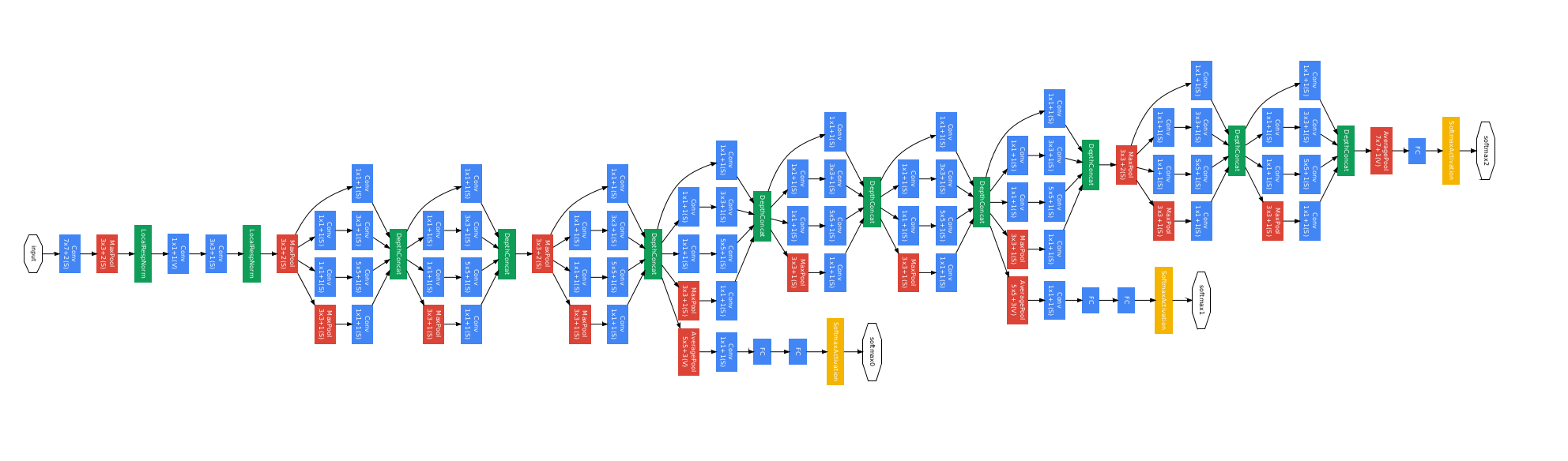
We will move to another model, Convolutional Neural Networks (or CNN). This model is way fitter to process images as its structure acknowledges the context we’re operating with and is therefore stronger at detecting visual patterns than a simple neural network. The following picture depicts a simple Convolutional Neural Network model:

We’ll try to briefly explain what each layer does, with a graphical support.
Input Layer
 The input layer is not a flat list of neurons anymore but rather a matrix. The spatial information is hence preserved and this is obviously crucial when dealing with images.
Shared Weights
 In convolutional neural network, weights and other parameters are shared between each so-called map. This significantly reduces the total number of parameters in the neural network.
Convolutional Layers
 A convolutional layer works in such a way that each neuron will produce the result of a convolution function applied to its local receptive field. Differently from the fully connected layers, a neuron in a convolutional layer is only connected to a small region of its input layer, usually a n x n matrix. This setting, together with the shared weights condition we discussed earlier, basically means that every neuron in such a layer will be trained to look for the same feature in different regions of the image, which is why this structure is referred to as feature map. This a powerful characteristic yet limiting since it only allows for one feature to be searched, be it vertical edges, horizontal edges and so on. To counterbalance this limitation, a convolutional layer is usually made up of many feature maps.
Pooling Layer
 The purpose of a pooling layer is to condense the activation output from the previous layer. It will output a function computed on the outputs of a cluster from neurons of the previous layer, causing the pooling layer to be significantly smaller than the previous one. Typical examples are max-pooling, where the maximum is returned or average-pooling, which is also pretty self-explanatory.
Output Layer
 Finally the output is flattened and processed through a softmax function or the likes in order to make the desired prediction.
CNN in practice
We will see that Keras provides remarkably intuitive APIs to compose a Convolutional Neural Network. First, let’s prepare our data to be fed to the CNN. Remember that this is the shape of our data as of right now:
X_train.shape
(60000, 784)
whereas for a CNN we would use an actual image with a matrix strucutre. Let’s reshape the input data to conform the shape (width, height, depth). In our case, the depth will be equal to 1 since we’re dealing with grayscales.
X_train = X_train.reshape((-1,28,28,1))
X_test = X_test.reshape((-1,28,28,1))
X_train.shape
(60000, 28, 28, 1)
Let’s import the necessary libraries
from keras.models import Model
from keras.layers import Input, Convolution2D, MaxPooling2D,Flatten
Let’s build the CNN. One of the upside of Keras is being able to write code which is pretty self-explanatory. We will build the model by adding several convolutional layers (Convolution2D), max-pooling layers (MaxPooling2D) and Dropout layers.
In the final stage, we will need to Flatten the output, then make it go through a fully connected layer (Dense), another dropout layer and finally a softmax layer to obtain the final probabilities.
inp = Input(shape=(28, 28,1))

conv_1 = Convolution2D(32, (3, 3), padding='same', activation='relu')(inp)
conv_2 = Convolution2D(32, (3, 3), padding='same', activation='relu')(conv_1)
pool_1 = MaxPooling2D(pool_size=(2, 2))(conv_2)
drop_1 = Dropout(0.5)(pool_1)

conv_3 = Convolution2D(64, (3, 3), padding='same', activation='relu')(drop_1)
conv_4 = Convolution2D(64, (3, 3), padding='same', activation='relu')(conv_3)
pool_2 = MaxPooling2D(pool_size=(2, 2))(conv_4)
drop_2 = Dropout(0.25)(pool_2)

flat = Flatten()(drop_2)
hidden = Dense(512, activation='relu')(flat)
drop_3 = Dropout(0.25)(hidden)
out = Dense(10, activation='softmax')(drop_3)
And build a model, simply by specifying its inputs and outputs
model = Model(inputs=inp, outputs=out)

model.compile(loss='categorical_crossentropy',
              optimizer='adam',
              metrics=['accuracy'])
history_cnn = model.fit(X_train, y_train_1h,
          batch_size=32, epochs=20,
          verbose=1, validation_split=0.1)
Train on 54000 samples, validate on 6000 samples
Epoch 1/20
54000/54000 [==============================] - 16s - loss: 0.4549 - acc: 0.8331 - val_loss: 0.2875 - val_acc: 0.8992
Epoch 2/20
54000/54000 [==============================] - 16s - loss: 0.2881 - acc: 0.8945 - val_loss: 0.2491 - val_acc: 0.9062
[...]
Epoch 19/20
54000/54000 [==============================] - 16s - loss: 0.1167 - acc: 0.9561 - val_loss: 0.2367 - val_acc: 0.9323
Epoch 20/20
54000/54000 [==============================] - 16s - loss: 0.1164 - acc: 0.9570 - val_loss: 0.2361 - val_acc: 0.9340
Let’s run a classification report
predicted_probabilities = model.predict(X_test)
cnn_predicted = predicted_probabilities.argmax(axis=-1)

print(metrics.classification_report(y_test, cnn_predicted,target_names=clothes_labels))
             precision    recall  f1-score   support

T-shirt/top       0.91      0.88      0.89      1000
    Trouser       0.99      0.99      0.99      1000
   Pullover       0.93      0.87      0.90      1000
      Dress       0.93      0.96      0.94      1000
       Coat       0.89      0.92      0.90      1000
     Sandal       1.00      0.99      0.99      1000
      Shirt       0.80      0.83      0.81      1000
    Sneaker       0.97      0.97      0.97      1000
        Bag       1.00      0.99      0.99      1000
 Ankle boot       0.97      0.98      0.98      1000

avg / total       0.94      0.94      0.94     10000
With a relatively simple model (cnn-wise), we already achieved incredible performances! It’s important to higlight how half of the categories are actually close to perfect scores (more than 0.97 on all metrics), whereas the shirt class is actually dragging the overall performance down, with no score higher than 0.82.
Chart time
It’s time to build up some charts and higlights our results. First, it could be interesting to look at the accuracy and loss progression through time.
%matplotlib inline
import matplotlib.pyplot as plt
f, (ax1, ax2) = plt.subplots(2,1, sharex=True, figsize=(10,8))
plt.xlabel('epochs')
ax1.plot(history_cnn.history['acc'])
ax1.plot(history_cnn.history['val_acc'])
ax1.set_ylabel('accuracy')
ax1.legend(['train', 'validation'], loc='upper left')

ax2.plot(history_cnn.history['loss'])
ax2.plot(history_cnn.history['val_loss'])
ax2.set_ylabel('loss')
ax2.legend(['train', 'validation'], loc='upper left')
plt.show();

This charts shows us that, while we achieved some good results on the training set, the generalization isn’t getting any better on the validation set, therefore our model could probably benefit from some more regularization but this isn’t the purpose of this post so we won’t dig any deeper in that direction.
Model scores comparison
We will quickly compare the Feed-Forward Neural Networks’ scores with Convolutional Neural Networks’ scores on a bar chart. In order to do this, we need to compute our desired scores:
from sklearn.metrics import f1_score, recall_score, matthews_corrcoef, precision_score

predictions = [nn_predicted,cnn_predicted]

scores = {}
scores['f1'] = []
scores['recall'] = []
scores['precision'] = []

for prediction in predictions:
    scores['f1'].append(f1_score(y_test, prediction,average=None))
    scores['recall'].append(recall_score(y_test, prediction,average=None))
    scores['precision'].append(precision_score(y_test, prediction,average=None))
Initialize a few support variables, code an helper function to setup the chart parameters.
import seaborn as sns
import numpy as np
sns.set(rc={"figure.figsize": (20, 12)})
sns.set_style("whitegrid")
colors = sns.color_palette()
clothes_range = np.arange(10)
bar_width = .4

def drawScores(metric):
    fig, ax = plt.subplots()
    plt.title(metric.upper(), fontsize=30, fontweight='bold', y=1.08)
    ax.bar(clothes_range, scores[metric][0], bar_width, label='FFNN')
    ax.bar(clothes_range + bar_width, scores[metric][1], bar_width, label='CNN')
    plt.xticks(clothes_range+bar_width/2, clothes_labels, fontsize = 16)
    plt.yticks(np.arange(0, 1.0, 0.02))
    plt.ylim([.5,1.])
    legend = plt.legend(frameon = 1, fontsize=20)
    frame = legend.get_frame()
    frame.set_color('white')
    frame.set_edgecolor('black')
    plt.show()
We will only draw the upper half of the chart, since none of our scores goes below 0.5 and that cut allows for a more focused visualization.
drawScores('f1')

drawScores('recall')

drawScores('precision')

The results are very similar, these charts highlight the remarkable performance gap between a traditional neural network and a convolutional neural network. Some of the worst-performing scores see a striking improvement when analyzed by a CNN, which practically never goes below 0.8.
Conclusions
This small but significant example tells us a few important things. First of all, it is yet another showcase of the power of machine learning. On the other hand it also tells us that, while machine learning is so amazing because it learns by itself, it gets much better at doing so when the one guiding is able to point it in the right direction. Being able to understand your context, analyse it and tweak these amazingly smart tools to adapt to this knowledge it’s the key to unlock the full potential of machine and deep learning. And once you do that, it truly is a marvel to witness.
Photo by NordWood Themes on Unsplash